Chapter 6:
Quantifying Residuals and Variance
in the Commercial Sector
Summary
This chapter details residual measurements from the difference of differences calculations specific to different business types in MCE service territory. These results provide a foothold for measuring the difference in consumption that could be expected due to COVID impacts and other exogenous factors when using the following measurement strategies:
Summary results from this experiment are provided in Table 5:
Table 5
This chapter details residual measurements from the difference of differences calculations specific to different business types in MCE service territory. These results provide a foothold for measuring the difference in consumption that could be expected due to COVID impacts and other exogenous factors when using the following measurement strategies:
- No comparison group
- A randomly selected comparison group of commercial customers
- A comparison group of similar business type
Summary results from this experiment are provided in Table 5:
Table 5
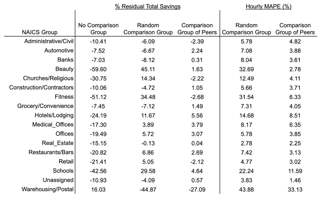
Without a comparison group, the residuals of the total savings calculations ranged from -60% to 16% across different business types. Taking Offices as an example, without a comparison group we observe a 19.5% difference between forecasted and actual energy consumption using a standard CalTRACK savings calculation. With the exception of the Warehousing/Postal and Banks NAICS groups, incorporating a randomly selected comparison group consistently reduced the residual, often significantly. However, most sectors still exhibited a greater than 5% difference and a number of subsectors had residuals between 10 - 45%. When we introduced a comparison group consisting of business type peers, major improvements could be seen in every sector.
Looking at the Restaurant/Bars subsector, we see that without a comparison group, one would expect a residual of 21% in a savings measurement. A randomly selected comparison group reduces the residual to 7% and a reduction to under 3% is achieved by applying a comparison group of peers.
Similar improvements were observed in the hourly MAPE. When shifting from a randomly selected comparison group to a comparison group of peers, MAPE improved for all 17 NAICS groups. Continuing with the Restaurants/Bars example, MAPE is reduced from 7.4% to 3.1% in the hourly measurement.
One may expect that, as is done in stratified sampling, selection of comparison group meters based on common consumption characteristics would yield improvement over random sampling. For this to be the case particular baseline-period usage patterns would need to be identified that are strongly correlated with the energy consumption changes due to COVID. We have tested this possibility across a range of potential stratification parameters by first measuring meter-level COVID impacts and then gauging the degree to which many distinct usage parameters are correlated with changes in usage attributable to COVID. Results are given in Table 6.
Table 6
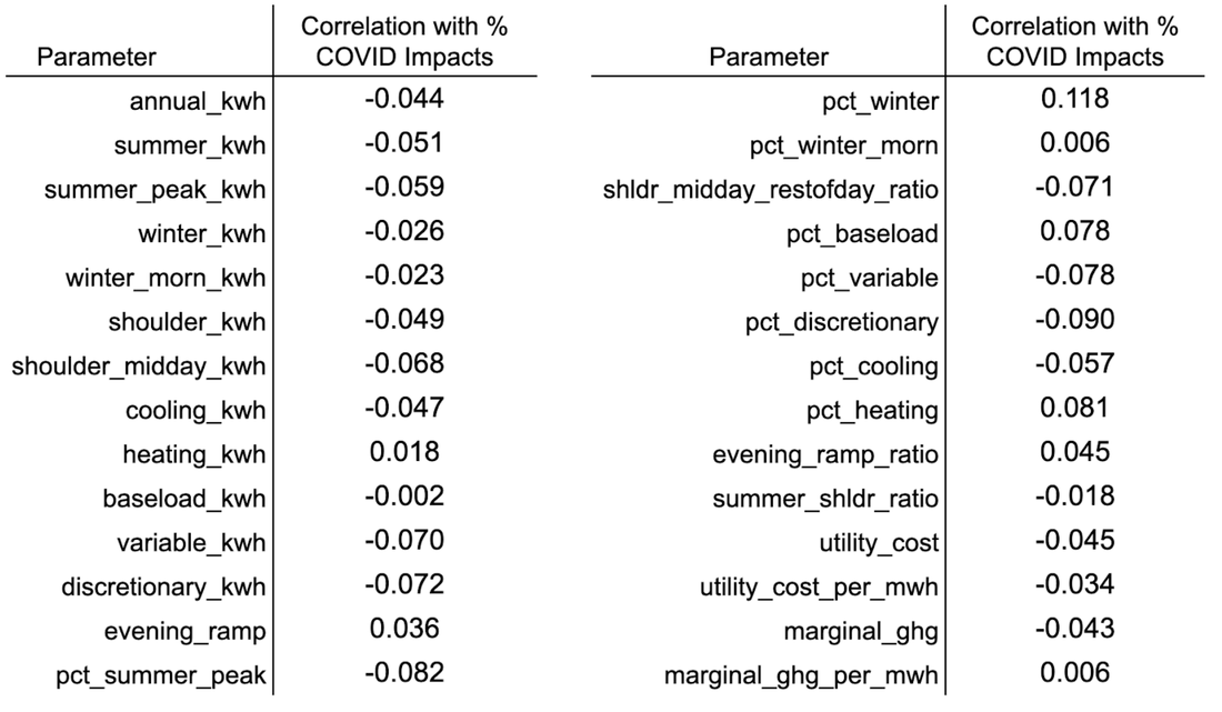
While there are some interesting patterns in these results, the key takeaway is that none of these various 28 parameters, all computed from pre-COVID data, show a strong enough correlation with COVID impacts to warrant additional investigation.
Experimental Details
Similar to the residential experiments of Chapter 5, the following stepwise analysis was conducted to gauge the degree of residual in a % difference of differences calculation due to COVID.
- Hourly CalTRACK 2.0 calculations were performed on all commercial meters in MCE territory using the timeline of Figure 1.
- Were solar customers (identified by rate code or the presence of negative meter readings).
- Had fewer than 329 days with at least one meter reading in the baseline period.
- Had more than 15% of hours with null meter readings across the days in the baseline period with at least one meter reading.
- Had fewer than 90% of days in the reporting period with at least one meter reading.
- Had more than 15% of hours with null meter readings across the days in the reporting period with at least one meter reading.
- Remaining meters were randomly split into two equal subgroups of equivalent size (12,203 meters each).
- The first of these groups was always used as the random sample.
- Each NAICS group was also randomly split into two equivalent samples.
- When computing the difference of differences calculation for a random sample vs. NAICS group, the first random sample was tested against the first NAICS subgroup. There will be a small degree of overlap between these two groups but this overlap should be 10% or less in every group except “Unassigned.”
- When computing the difference of differences calculation for a NAICS group vs a peer group, the random samples from step 4 are tested against one another. There is no overlap between these groups.
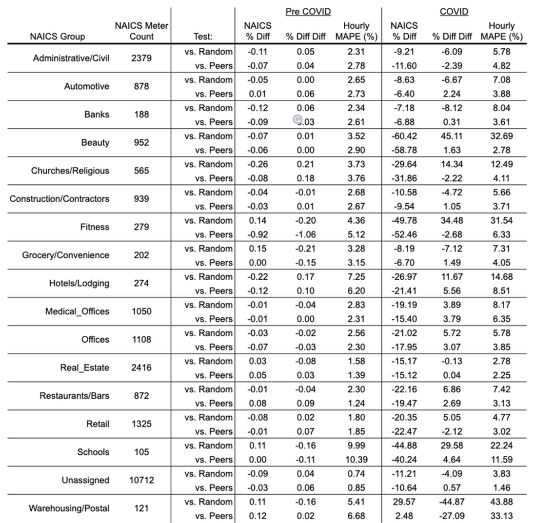
Table 7 gives results (% Difference for the NAICS groups, % Difference of Differences for NAICS Group vs. Random and NAICS vs. Peers) for both the pre-COVID period and COVID periods.
Table 7
Appendix C provides detailed results and figures for every test case summarized.