Chapter 5:
Quantifying Residuals and Variance
in the Residential Sector
This chapter details residual measurements from difference of differences calculations for MCE’s residential sector. We describe the difference in consumption between forecasted and observed as a residual, which can be understood as the combination of exogenous factors and statistical noise after weather-normalizing the data. Note that a value of percentage residual is in reference to total consumption. Unintended residuals between program participants and potential comparison groups could arise due to different geographic locations, different usage patterns and other factors such as income and demographic characteristics. In this chapter we focus on geography and usage patterns with the goal of understanding to what extent misalignments between treatment and comparison groups would be expected to yield savings uncertainty and variance on account of COVID.
Geography
This section summarizes results for the geographic trials. Random samples were taken from each of the six largest cities in MCE service territory. These cities cover a diverse range of climates as well as income and demographic characteristics. For instance, the city of Richmond has nearly double the proportion of low-income residents than Napa, and has far lower average usage than in MCE territory as a whole. For each of these samples we assess residuals in the difference of differences calculation when the following strategies are employed for comparison group selection:
Figure 14 gives an example of the load shape differences observed between one of these cities. The average daily load shape of an MCE residential meter is shown in blue (circles) with the average daily load shape of a residential Pittsburgh meter shown in green (triangles).
Geography
This section summarizes results for the geographic trials. Random samples were taken from each of the six largest cities in MCE service territory. These cities cover a diverse range of climates as well as income and demographic characteristics. For instance, the city of Richmond has nearly double the proportion of low-income residents than Napa, and has far lower average usage than in MCE territory as a whole. For each of these samples we assess residuals in the difference of differences calculation when the following strategies are employed for comparison group selection:
- No comparison group
- A randomly selected comparison group of residential customers from across MCE territory
- A randomly selected comparison group of non-overlapping customers from the same city.
Figure 14 gives an example of the load shape differences observed between one of these cities. The average daily load shape of an MCE residential meter is shown in blue (circles) with the average daily load shape of a residential Pittsburgh meter shown in green (triangles).
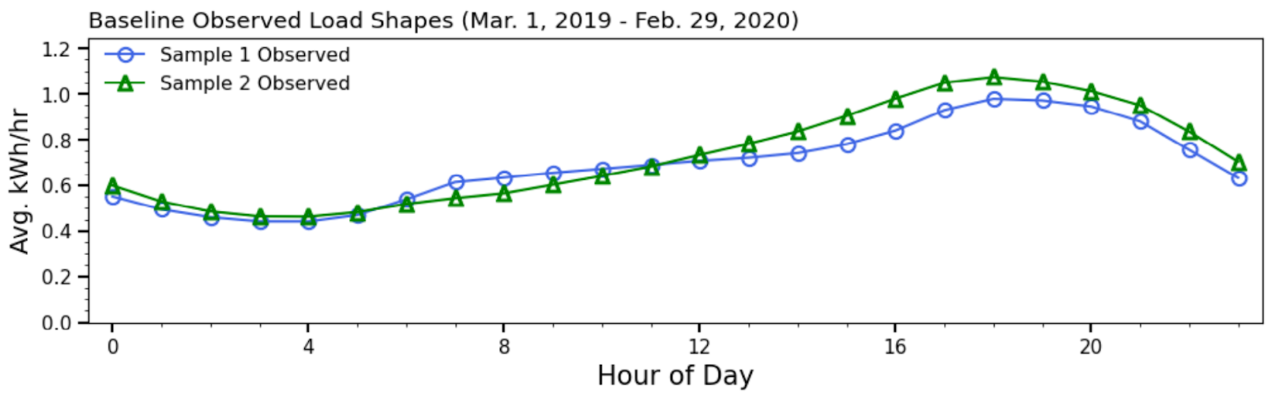
Figure 14: Average daily load shape of a residential non-solar MCE meter (blue circles) and a residential non-solar MCE meter in Pittsburgh (green triangles).
The difference in load shape may or may not lead to a COVID-related residual in % difference of differences calculation. Summary results from this experiment are provided in Table 2 for both residuals present in a total savings calculation, and the mean absolute percentage error (MAPE) observed in the measurement of hourly load impacts.
Table 2
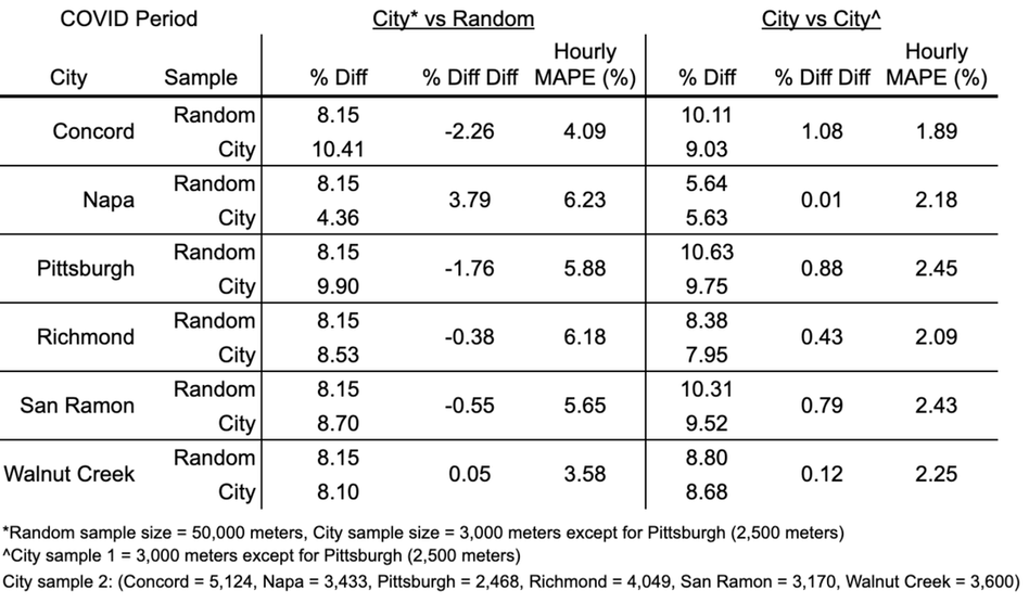
Without a comparison group, residuals in a total savings calculation ranged from -5.6% to 10.6% across different cities. When comparing a random sample from MCE’s entire service territory, residuals ranged from near 0 (Walnut Creek) to 3.8% (Napa). This degree of uncertainty may be acceptable to program administrators for whom measuring annual savings is the most important consideration. Despite a smaller sample size, a reduction of residuals is observed in most cases when a comparison group is formulated by sampling from the same city. In all cases investigated here, the residual in the COVID-period total difference of differences calculation was less than 1.1% when selecting treatment and comparison randomly from the same city.
For program administrators seeking reliability in the hourly calculation of load impacts, these results show a clear advantage of pulling the comparison group from the same geographic location. Mean Absolute Percent Error (MAPE) in the hourly difference of differences measurements was below 2.5% for each within-city trial but ranged from 3.6% to 6.2% when comparing a specific city to the territory-wide sample. When moving from a sector-wide to a city-specific comparison group, the improvement in hourly measurements is evident in the data provided in Appendix B.
Usage Characteristics
Along with geographic considerations, demand-side programs often target customers based on specific usage patterns. For example, a demand response program would likely seek customers who exhibit high peak period usage. Customers with different usage patterns may respond differently to COVID and if not accounted for these differences can lead to bias in a difference of differences calculation.
In this section we establish samples of MCE residential customers with systematic differences in particular usage characteristics, measured during the pre-COVID-period. For each sample, we then test the following comparison group scenarios:
Table 3 details the selection schemes explored here.
Table 3
For program administrators seeking reliability in the hourly calculation of load impacts, these results show a clear advantage of pulling the comparison group from the same geographic location. Mean Absolute Percent Error (MAPE) in the hourly difference of differences measurements was below 2.5% for each within-city trial but ranged from 3.6% to 6.2% when comparing a specific city to the territory-wide sample. When moving from a sector-wide to a city-specific comparison group, the improvement in hourly measurements is evident in the data provided in Appendix B.
Usage Characteristics
Along with geographic considerations, demand-side programs often target customers based on specific usage patterns. For example, a demand response program would likely seek customers who exhibit high peak period usage. Customers with different usage patterns may respond differently to COVID and if not accounted for these differences can lead to bias in a difference of differences calculation.
In this section we establish samples of MCE residential customers with systematic differences in particular usage characteristics, measured during the pre-COVID-period. For each sample, we then test the following comparison group scenarios:
- No comparison group
- A randomly selected comparison group of residential customers from across MCE territory
- A randomly selected comparison group of customers who meet the same consumption-based selection criteria.
Table 3 details the selection schemes explored here.
Table 3
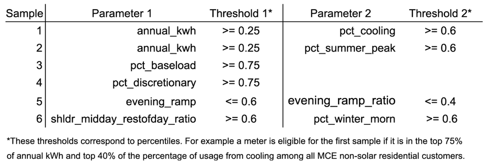
Figure 15 gives an example of the load shape differences observed between an average MCE customer and a customer in Sample 1 (Table 3). The average daily load shape of an MCE residential customer is shown in blue (circles) with the average daily load shape of a customer in Sample 1 in green (triangles).
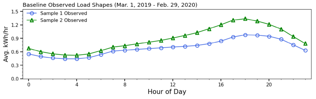
Figure 15: Average load shape of a residential non-solar MCE meter (blue circles) and a residential non-solar MCE meter in the top 75% and top 40% of all residential meters in annual usage and the percent of usage from cooling.
Table 4 provides a summary of results for these comparison group tests.
Table 4
Table 4 provides a summary of results for these comparison group tests.
Table 4
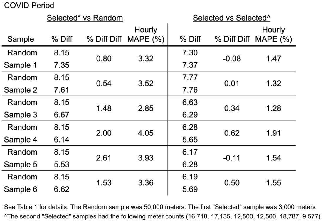
Without a comparison group, residuals ranged from -5.7% to 7.8% across the different samples of Table 4. Interestingly, none of these samples exhibited greater impacts from COVID than the territory-wide random selection (8.2%). When using this territory-wide random sample as a comparison group, residuals in the difference of differences calculation ranged from 0.5% to 2.6%. Reminiscent of the geographic samples, despite smaller sample sizes, a reduction in residuals is observed in all cases when a comparison group is formulated by sampling with the same selection criteria. In the current cases, residuals in the COVID-period total difference of differences calculation were less than 0.6% across the board when doing so.
Significant improvements in the hourly MAPE are observed when employing the same usage-based selection criteria between samples. With the random comparison group approach the MAPE ranged from 2.9% to 4.1% compared to 1.3% to 1.9% when applying the same selection requirements.
Experimental Details
The following stepwise analysis was conducted to produce the results above and gauge the degree of residual in a % difference of differences calculation due to COVID.
- Were solar customers (identified by rate code or the presence of negative meter readings).
- Had a total annual consumption in the baseline period greater than 50 MWh.
- Had fewer than 329 days with at least one meter reading in the baseline period.
- Had more than 15% of hours with null meter readings across the days in the baseline period with at least one meter reading.
- Had fewer than 90% of days in the reporting period with at least one meter reading.
- Had more than 15% of hours with null meter readings across the days in the reporting period with at least one meter reading.
Significant improvements in the hourly MAPE are observed when employing the same usage-based selection criteria between samples. With the random comparison group approach the MAPE ranged from 2.9% to 4.1% compared to 1.3% to 1.9% when applying the same selection requirements.
Experimental Details
The following stepwise analysis was conducted to produce the results above and gauge the degree of residual in a % difference of differences calculation due to COVID.
- Hourly CalTRACK 2.0 calculations were performed on all residential meters in MCE territory using the timeline of Figure 1.
- Were solar customers (identified by rate code or the presence of negative meter readings).
- Had a total annual consumption in the baseline period greater than 50 MWh.
- Had fewer than 329 days with at least one meter reading in the baseline period.
- Had more than 15% of hours with null meter readings across the days in the baseline period with at least one meter reading.
- Had fewer than 90% of days in the reporting period with at least one meter reading.
- Had more than 15% of hours with null meter readings across the days in the reporting period with at least one meter reading.
- Usage-based stratification parameters were computed for all meters.
- The remaining meters were randomly split into two subgroups of equivalent size (50,000 meters each).
- When testing against a territory-wide random sample, the first of these groups was always used as the random sample and the second group always served to furnish the city- or usage-based samples.
- When testing samples with the same selection criteria, all qualifying meters from the first group were taken as the first sampler esiduals, and 3,000 random meters meeting the selection criteria were pulled from the second group.