Chapter 3:
Recommended Sampling Methods
In the evaluation of demand-side energy programs, many comparison group sampling strategies have been developed and deployed. A full review of each approach is beyond this work, but common categories include random sampling, stratified sampling, future participants, and site-based matching. In developing recommendations for standardized methods to enable meter-based pay-for-performance programs, the following requirements are critical:
In addition to these conditions, the following recommendations are rooted in the testing of many different comparison group scenarios, which are detailed in Chapters 5 and 6 and complimentary appendices B and C.
While it can be desirable to have a single approach applied to all possible scenarios, our observations throughout the research and development phase of this effort have led us to an additional consideration:
6. Methods must be appropriate for the specific use case.
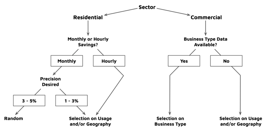
In particular, we have observed that while individual customers in the residential sector have exhibited a wide range of changes to energy consumption due to COVID, the distributions of meter-level COVID impacts have tended to be relatively consistent among different groups of customers. This is in contrast to the commercial sector, where very clear and substantive differences are observed between different customer segments. As a result, when a measurement of total monthly or annual savings is the goal, random sampling may be a more appropriate and reliable approach for a residential program than for a program serving a specific commercial segment.
When hourly measurements or greater precision in total savings are needed, Chapter 5/Appendix B shows that hourly measurements benefit from a comparison group selected based on additional criteria, including geographic location and usage characteristics. These results lead us to the following decision tree in the initial assessment of the type of sampling approach that should be employed for specific use cases:
- Methods need to enable sampling based either on a program’s forecasted participation or on the population of actual treated customers.
- Methods and required data must allow for tracking of a live program.
- Methods must produce comparison groups amenable to statistical equivalence computations against the corresponding treatment groups.
- Methods must result in as few subjective inputs and decisions as possible, even if that leads to greater complexity in the sampling execution and code.
- Methods must not be prohibitively complex or computationally expensive to implement.
In addition to these conditions, the following recommendations are rooted in the testing of many different comparison group scenarios, which are detailed in Chapters 5 and 6 and complimentary appendices B and C.
While it can be desirable to have a single approach applied to all possible scenarios, our observations throughout the research and development phase of this effort have led us to an additional consideration:
6. Methods must be appropriate for the specific use case.
In particular, we have observed that while individual customers in the residential sector have exhibited a wide range of changes to energy consumption due to COVID, the distributions of meter-level COVID impacts have tended to be relatively consistent among different groups of customers. This is in contrast to the commercial sector, where very clear and substantive differences are observed between different customer segments. As a result, when a measurement of total monthly or annual savings is the goal, random sampling may be a more appropriate and reliable approach for a residential program than for a program serving a specific commercial segment.
When hourly measurements or greater precision in total savings are needed, Chapter 5/Appendix B shows that hourly measurements benefit from a comparison group selected based on additional criteria, including geographic location and usage characteristics. These results lead us to the following decision tree in the initial assessment of the type of sampling approach that should be employed for specific use cases:
Program Forecasting Stage
It will be advantageous for many meter-based pay-for-performance programs to have a comparison group established at the outset based on a forecasted population of participants. The forecast-based comparison group will help get the program on track for savings calculations and aggregator performance payments. As it cannot be known in the forecasting phase which specific customers will ultimately participate, some common comparison group strategies, including individual site-based matching and future participants, will not be possible.
At this point, according to the decision tree above, either a random sampling or proportional sampling scheme can be deployed. In either case, it will be important that the comparison pool is limited to customers that meet the same data sufficiency and program eligibility considerations required for participating customers. For instance, if the program requires participating customers to have a minimum annual usage of 1 MWh and no solar PV system, then the comparison pool should be screened for these criteria as well.
In the Residential sector, proportional sampling can be conducted on the basis of both geographic location and usage characteristics expected for program participants. If an efficiency program in Arizona wished to target high air conditioning users in the low elevation climate regions, proportional sampling could be done from these geographic areas and weighted to populations with high cooling loads observed at the meter. Chapter 5/Appendix B demonstrates how both geographic and usage-based sampling can reduce residuals in the calculation of load impacts, including on an hourly basis.
In the commercial sector, we observe that business type is the most reliable predictor of population-level consumption changes due to COVID. Therefore, our recommendation is to utilize business type (via NAICS code or other data sources) information as a selection parameter in the formulation of a comparison group wherever these data are available. For forecasting, the program administrator and aggregator should assess likely participating business types and formulate a comparison group based on the outcome of this process. Where business type information for the comparison pool is not available, sampling based on expected geographic location and customer usage characteristics can help to identify the most relevant comparison group. However, due to the high degree of variance in COVID impacts by economic sub-sector, where business type data are not available, program administrators and aggregators will face increased risk. In these cases, serving a wide variety of customers in the program can help mitigate risk.
Program Implementation Stage
After a program enters its enrollment phase, an actual participant group will emerge. Depending on the circumstances of the in-field program, this group may or may not align well with the forecast. Differences could emerge related to business type, geography, usage characteristics, or other important factors. In these cases, program administrators and aggregators may wish to reformulate the comparison group to better represent the actual program participation. This step can mitigate risk for both parties associated with a mismatched comparison group.
With COVID impacts driving the largest non-program changes in energy usage and business type being the best predictor of these changes, comparison group resampling for Commercial programs should be done first to ensure that the proportion of business types in the comparison group matches that of the treatment group. Given sufficient meters in the comparison pool, the comparison group can be further refined to best capture geographic and/or usage characteristics per the stratification methods detailed in the next section.
For the Residential sector, we recommend that resampling be done based on the stratified sampling approach described below.
Stratified Sampling
In stratified sampling, a comparison group is generated from a comparison pool by selectively eliminating members of the comparison pool until the remaining sample is representative of a treatment group. This elimination step is done on the basis of one or more characteristics that can be known or measured for all members of both treatment and comparison samples. In practice, stratification is done by identifying specific, quantifiable parameters of interest and then forming discrete bins based on the values of those parameters observed in the treatment group. Each customer is assigned to a single bin. The resulting counts within each bin determines the proportionality that must then be matched by sampling from the comparison pool.
Illustrative Example: Traditional Stratified Sampling
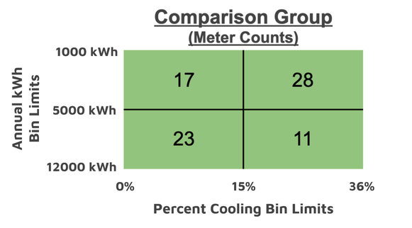
To illustrate the concepts of multidimensional stratified sampling based on usage characteristics, we consider the following treatment group and comparison pool where stratification is to be done based on the parameters of total annual kWh usage (annual_kwh) and the percentage of a customer’s usage from cooling (pct_cooling). To keep the example tractable, we split each parameter into just two bins, creating a total of four bins. The figure below shows how meters in the treatment group are assigned to bins given the indicated limits. A meter with 7,430 annual kWh and 11% cooling would be one of the 8 meters assigned to the lower-left bin.
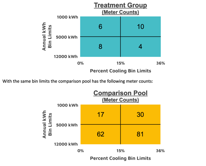
Comparing the fraction of meters in each bin, we see that the comparison pool differs from the treatment group:
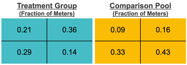
The job of stratified sampling is to create fractional parity between the treatment and comparison groups within each bin. Since the comparison pool is set, meters cannot be added to underrepresented bins. Instead, meters must be eliminated from bins that are oversampled compared to the treatment group. For any binning scheme, a “limiting bin” will emerge corresponding to the most undersampled bin in the comparison pool. The limiting bin is determined by taking the ratio of population in the comparison pool vs. treatment group for each bin and locating the minimum. In the current example, this step results in the following:
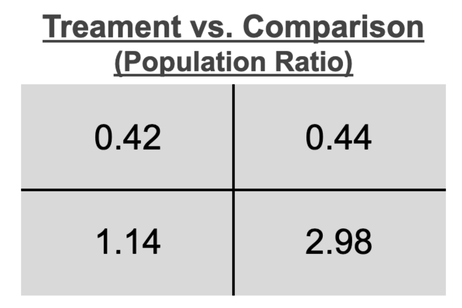
With the upper left bin having the lowest ratio, we must eliminate meters from each of the other bins until all bins have a 1.0 ratio between treatment and comparison groups. This can be done in one step by dividing the comparison pool meter count in the limiting bin by the treatment group fraction of meters in the limiting bin and then multiplying by the fraction of meters in the treatment group for each bin. Using the lower-left bin as an example:

Applying this procedure to all bins yields the following comparison group:
We see that in this case we have produced a proportional match in each bin by resampling a comparison pool of 190 meters to a comparison group of 79 meters.
It is important to note that achieving proportional binning does not equate to an unbiased sample, even when only considering the specific stratification parameters. In this example, it is possible that within the top bins the comparison pool is over-represented from 1000 to 3000 annual kWh and under-represented from 3000 to 5000 annual kWh. In this case, it may be necessary to move to three or more bins for annual kWh to force a more granular sampling.
This is a key concept we will return to below. Stratified sampling can be made more precise with enhanced granularity - increased number of parameters and/or an increased number of bins per parameter. However, as with many other sampling techniques, stratified sampling is ultimately constrained by the total number of meters in the comparison pool and the number of meters needed for a comparison group. With a smaller comparison pool, fewer bins across fewer parameters can be utilized before eliminating too many meters to meet the minimum requirement for the final comparison group.
Enhanced Stratified Sampling
How does one define the success or failure of a comparison group formed by stratified sampling or any other method for that matter? Is a comparison group reliable and representative because we achieve proportional binning for certain parameters in relation to a treatment group? What is the best or proper way to gauge statistical similarity between a comparison group and a treatment group?
Stratified sampling is a means to an end. The ultimate goal is a comparison group that is the most representative of a treatment group and with enough statistical power as to not introduce undue uncertainty into a savings measurement. To this end, stratified sampling is just a tool. A good proportional match for chosen stratification parameters does not guarantee that other important aspects of energy usage have been well emulated by the selected comparison group.
Many evaluators, including Recurve, have utilized individual site-based matching schemes in which each treatment meter is assigned one or more comparison group meters based on a direct measurement of usage. Site-based matching has been done in recent studies by minimizing a Euclidean distance metric computed across the baseline period monthly consumption for each comparison group meter tested against each treatment group meter. Though we are not recommending site-based matching here, the fact that this strategy focuses directly on the load profiles of treatment and comparison meters - and not isolated usage characteristics - is a highly attractive feature.
With these considerations in mind, we propose an advanced stratified sampling technique wherein optimization is not conducted by minimizing treatment vs. comparison discrepancies specific to the chosen stratification parameters themselves, but rather by optimizing the fit between the resultant load profiles. Therefore, instead of striving for statistical equivalence using a T-Test or KS-Test, or enforcing an optimization scheme on the stratification parameter distributions, we propose gauging the performance of a candidate stratified sampling scheme on its ability to minimize the discrepancy between treatment and comparison group load profiles.
Where only monthly data are available, the load profile has a maximum of 12 data points per customer per year. In contrast, with hourly data one could attempt to optimize across the entire 8,760 annual load shape, but this would be enormously expensive and not likely to yield significantly improved results compared to more aggregated options. With hourly data, we suggest that taking into account both seasonal and weekday vs. weekend differences is important beyond simply assessing an average 24-hour average daily load shape. Thus while 8,760 data points may be excessive, 24 cannot capture important comparative features. Instead, we recommend using average seasonal weekly load shapes for the summer, winter, and shoulder timeframes. The resulting 504 data point representation is nearly 20 times smaller than the full 8,760 profile yet retains the majority of relevant information.
In taking this approach it is important to guard against the potential pitfall that wildly disparate comparison group load shapes could simply average to produce a similar profile to an average treatment group load shape. Therefore, a straight least-squares optimization of an average comparison group load profile vs. an average treatment group load profile should be avoided. Instead, we recommend an approach in which each data point in the average load profile is broken into bins of equal proportion for both treatment and comparison groups. Considering a monthly load profile, the average January consumption for treatment and comparison group customers is split into bins by percentile. A treatment group of 250 meters can be ordered by January consumption and broken into 10 groups of 25 meters. The lowest usage group corresponds to the 0 - 10% decile and the highest usage group corresponds to the 90 - 100% decile. The exact same procedure for the comparison group yields a corresponding set of deciles. The average January usage for each decile in the treatment group forms a distribution that can be compared directly to the distribution produced from the comparison group. At this point a sum of squares computation can be performed across each decile. Finer binning can also be conducted if computational resources allow.
Continuing with the monthly example, repeating this process for each month yields 12 sums of squares that can be summed for a total sum of squares value, which represents the degree of distributional similarity between treatment and comparison groups. As described above, when hourly data are available, seasonal load shapes can be the focus of this computation. With this approach we can ensure that an average comparison group load profile does not appear to be a good representation of a treatment group when the underlying usage distributions among component meters differ substantially.
In the next section we turn our attention to the automated development of candidate stratification schemes to be tested against a treatment group using the approach described here. The stratification scheme that produces the lowest value of the summed least-squares computation will be used to produce the comparison group.
Automating Generation of Candidate Stratification Schemes
In the illustrative example of Section A several areas of potential subjectivity are apparent:
The number of parameters
In considering the number of parameters it is important to understand why selecting many parameters is infeasible. In Section A we introduced the concept of a “limiting bin,” where the comparison pool is most underrepresented relative to a treatment group. As more parameters are added, the number of bins grows exponentially. Imagine adding parameters, each with only 2 bins. Each new parameter interacts with all other parameters, thereby doubling the number of total bins. Therefore, going from 2 to 3 parameters increases the number of bins from 4 to 8. But increasing from 6 to 7 parameters increases the number of bins from 64 to 128. As the number of bins increases, the probability that the limiting bin severely restricts the possible number of comparison meters increases as the comparison group is carved into finer and finer slices.
For most stratification schemes we expect that a maximum of three parameters can provide for sampling over several important aspects of customer usage while avoiding rapid over-binning. However, where sufficient data are available, there is no harm necessarily in moving to more parameters.
The choice of specific parameters
While at this point we do not offer concrete parameters for all use cases or code to automate parameter selection, we do provide the following considerations and guidance:
3, 4, 5. The number of bins, bin limits, and the number of comparison group meters
These items are interrelated and we cover them together. We have automated an optimized binning scheme with the following procedure:
i. For each parameter, the minimum of the lowest bin is set by the minimum value observed in the treatment group. Similarly, the maximum value of the highest bin is set by the maximum value observed in the treatment group.
ii. A minimum of 1 and maximum of 8 bins are allowed per stratification parameter.
iii. Beginning with a single bin for each parameter, every possible binning combination is scanned. For two parameters there are 64 possible binning arrangements [(1, 1), (1, 2), (2, 1), (2, 2)...(8, 8)].
iv. Depending on the size of the treatment group, scans are aborted for binning combinations that fail to yield a user-defined ratio of comparison group meters to treatment group meters. A minimum ratio of 4:1 is recommended for small Residential treatment groups (< 750 meters). For the Commercial sector this ratio will depend on the business type.
v. For binning combinations that yield a large number of meters, a random selection of available comparison pool meters is taken to meet a user-defined maximum. For both Residential and Commercial programs, a maximum value of at least 3,000 meters can help ensure uncertainty due to random variability in the comparison group is kept under +/- 2% in 90% of cases (see Fig. 7 of Chapter 2).
vi. All candidate comparison groups that pass the minimum threshold of step iv are passed to the sum of squares calculation described in Section IV.B.
vii. The final comparison group is selected based on the lowest sum of squares value computed as described in Section IV.B.
With the approaches described in this chapter, the establishment of comparison groups can be use-case specific and completed on the basis of a forecasted or actual treatment group. In the commercial sector the most important factor in achieving a comparison group capable of isolating program impacts and removing COVID impacts should focus first on building type wherever those data are available. In the Residential sector, geographic location and key usage patterns can serve as the basis for formulating comparison groups capable of reducing COVID-related residuals in a difference of differences calculation.
In both the Commercial and Residential sectors, where sampling stems from a program’s actual participant group, the enhanced stratified sampling methods of sections B and C are designed to strike a balance between the computational feasibility of stratified sampling and the advantages of direct load profile matching offered by site-based strategies. Where hourly data are available, an optimization conducted on seasonal weekly load shapes with largely independent stratification parameters that are representative of differences between a treatment group and comparison pool promises to produce comparison groups that can be used with confidence.
Example
As a test case for these methods we created a fake treatment group, which differed from the general population of MCE residential customers, and then executed each of the above steps to automatically select a comparison group. The treatment group was pulled from the first 50,000-meter sample described in the previous chapter with the following steps:
The binning scheme that yielded the lowest sum of squares across the 504 seasonal weekly load shape profile was 2 bins for annual kWh, 3 bins for percent summer peak, and 2 bins for the evening ramp ratio with a resulting 4,997 meters. This scheme improved the comparison pool sum of squares metric from 561 to 66 for the final comparison group.
The left-hand plot of Figure 10 shows the impact of stratification along each parameter that results from this three-dimensional binning scheme. The distribution of the comparison pool, shown in red, is significantly different, especially for the percent summer peak parameter, than those of the treatment group. After stratified sampling, clear improvements are observed across the board, though there is still some mismatch apparent in the lowest percent summer peak bin. This would likely be remedied with a higher limit on bins for this parameter.
It is important to note that achieving proportional binning does not equate to an unbiased sample, even when only considering the specific stratification parameters. In this example, it is possible that within the top bins the comparison pool is over-represented from 1000 to 3000 annual kWh and under-represented from 3000 to 5000 annual kWh. In this case, it may be necessary to move to three or more bins for annual kWh to force a more granular sampling.
This is a key concept we will return to below. Stratified sampling can be made more precise with enhanced granularity - increased number of parameters and/or an increased number of bins per parameter. However, as with many other sampling techniques, stratified sampling is ultimately constrained by the total number of meters in the comparison pool and the number of meters needed for a comparison group. With a smaller comparison pool, fewer bins across fewer parameters can be utilized before eliminating too many meters to meet the minimum requirement for the final comparison group.
Enhanced Stratified Sampling
How does one define the success or failure of a comparison group formed by stratified sampling or any other method for that matter? Is a comparison group reliable and representative because we achieve proportional binning for certain parameters in relation to a treatment group? What is the best or proper way to gauge statistical similarity between a comparison group and a treatment group?
Stratified sampling is a means to an end. The ultimate goal is a comparison group that is the most representative of a treatment group and with enough statistical power as to not introduce undue uncertainty into a savings measurement. To this end, stratified sampling is just a tool. A good proportional match for chosen stratification parameters does not guarantee that other important aspects of energy usage have been well emulated by the selected comparison group.
Many evaluators, including Recurve, have utilized individual site-based matching schemes in which each treatment meter is assigned one or more comparison group meters based on a direct measurement of usage. Site-based matching has been done in recent studies by minimizing a Euclidean distance metric computed across the baseline period monthly consumption for each comparison group meter tested against each treatment group meter. Though we are not recommending site-based matching here, the fact that this strategy focuses directly on the load profiles of treatment and comparison meters - and not isolated usage characteristics - is a highly attractive feature.
With these considerations in mind, we propose an advanced stratified sampling technique wherein optimization is not conducted by minimizing treatment vs. comparison discrepancies specific to the chosen stratification parameters themselves, but rather by optimizing the fit between the resultant load profiles. Therefore, instead of striving for statistical equivalence using a T-Test or KS-Test, or enforcing an optimization scheme on the stratification parameter distributions, we propose gauging the performance of a candidate stratified sampling scheme on its ability to minimize the discrepancy between treatment and comparison group load profiles.
Where only monthly data are available, the load profile has a maximum of 12 data points per customer per year. In contrast, with hourly data one could attempt to optimize across the entire 8,760 annual load shape, but this would be enormously expensive and not likely to yield significantly improved results compared to more aggregated options. With hourly data, we suggest that taking into account both seasonal and weekday vs. weekend differences is important beyond simply assessing an average 24-hour average daily load shape. Thus while 8,760 data points may be excessive, 24 cannot capture important comparative features. Instead, we recommend using average seasonal weekly load shapes for the summer, winter, and shoulder timeframes. The resulting 504 data point representation is nearly 20 times smaller than the full 8,760 profile yet retains the majority of relevant information.
In taking this approach it is important to guard against the potential pitfall that wildly disparate comparison group load shapes could simply average to produce a similar profile to an average treatment group load shape. Therefore, a straight least-squares optimization of an average comparison group load profile vs. an average treatment group load profile should be avoided. Instead, we recommend an approach in which each data point in the average load profile is broken into bins of equal proportion for both treatment and comparison groups. Considering a monthly load profile, the average January consumption for treatment and comparison group customers is split into bins by percentile. A treatment group of 250 meters can be ordered by January consumption and broken into 10 groups of 25 meters. The lowest usage group corresponds to the 0 - 10% decile and the highest usage group corresponds to the 90 - 100% decile. The exact same procedure for the comparison group yields a corresponding set of deciles. The average January usage for each decile in the treatment group forms a distribution that can be compared directly to the distribution produced from the comparison group. At this point a sum of squares computation can be performed across each decile. Finer binning can also be conducted if computational resources allow.
Continuing with the monthly example, repeating this process for each month yields 12 sums of squares that can be summed for a total sum of squares value, which represents the degree of distributional similarity between treatment and comparison groups. As described above, when hourly data are available, seasonal load shapes can be the focus of this computation. With this approach we can ensure that an average comparison group load profile does not appear to be a good representation of a treatment group when the underlying usage distributions among component meters differ substantially.
In the next section we turn our attention to the automated development of candidate stratification schemes to be tested against a treatment group using the approach described here. The stratification scheme that produces the lowest value of the summed least-squares computation will be used to produce the comparison group.
Automating Generation of Candidate Stratification Schemes
In the illustrative example of Section A several areas of potential subjectivity are apparent:
- The number of parameters
- The choice of specific parameters
- The number of bins
- Where to place the bin limits
- The number of comparison group meters to select
The number of parameters
In considering the number of parameters it is important to understand why selecting many parameters is infeasible. In Section A we introduced the concept of a “limiting bin,” where the comparison pool is most underrepresented relative to a treatment group. As more parameters are added, the number of bins grows exponentially. Imagine adding parameters, each with only 2 bins. Each new parameter interacts with all other parameters, thereby doubling the number of total bins. Therefore, going from 2 to 3 parameters increases the number of bins from 4 to 8. But increasing from 6 to 7 parameters increases the number of bins from 64 to 128. As the number of bins increases, the probability that the limiting bin severely restricts the possible number of comparison meters increases as the comparison group is carved into finer and finer slices.
For most stratification schemes we expect that a maximum of three parameters can provide for sampling over several important aspects of customer usage while avoiding rapid over-binning. However, where sufficient data are available, there is no harm necessarily in moving to more parameters.
The choice of specific parameters
While at this point we do not offer concrete parameters for all use cases or code to automate parameter selection, we do provide the following considerations and guidance:
- Parameters should be chosen that are relevant to the program because they are likely to be sensitive to the specific intervention. For instance, if a program plans to replace inefficient gas furnaces, then choosing parameters related to space heating gas usage, such as temperature-dependent or winter gas consumption, would help ensure that the comparison group reflects the usage characteristics most likely to showcase program influence.
- Parameters should be chosen that are not themselves highly correlated. For MCE’s Residential customer base, we have measured the correlation coefficient between summer and annual electricity consumption to be 0.94. Thus using both of these metrics as stratification parameters would offer very little additional information.
- A combination of dimensioned and dimensionless metrics should be used. A dimensioned parameter will reflect total consumption while a dimensionless parameter will allow a focus on critical aspects of consumption that are more related to how customers are using energy instead of just serving as another gauge of how much they are consuming. This recommendation is related to the last point. The correlation coefficient between annual kWh and cooling kWh is 0.56 but is only 0.15 between annual kWh and percent cooling. If a program is focused on air conditioning, the latter combination of parameters would provide for a higher level of distinction.
3, 4, 5. The number of bins, bin limits, and the number of comparison group meters
These items are interrelated and we cover them together. We have automated an optimized binning scheme with the following procedure:
i. For each parameter, the minimum of the lowest bin is set by the minimum value observed in the treatment group. Similarly, the maximum value of the highest bin is set by the maximum value observed in the treatment group.
ii. A minimum of 1 and maximum of 8 bins are allowed per stratification parameter.
iii. Beginning with a single bin for each parameter, every possible binning combination is scanned. For two parameters there are 64 possible binning arrangements [(1, 1), (1, 2), (2, 1), (2, 2)...(8, 8)].
iv. Depending on the size of the treatment group, scans are aborted for binning combinations that fail to yield a user-defined ratio of comparison group meters to treatment group meters. A minimum ratio of 4:1 is recommended for small Residential treatment groups (< 750 meters). For the Commercial sector this ratio will depend on the business type.
v. For binning combinations that yield a large number of meters, a random selection of available comparison pool meters is taken to meet a user-defined maximum. For both Residential and Commercial programs, a maximum value of at least 3,000 meters can help ensure uncertainty due to random variability in the comparison group is kept under +/- 2% in 90% of cases (see Fig. 7 of Chapter 2).
vi. All candidate comparison groups that pass the minimum threshold of step iv are passed to the sum of squares calculation described in Section IV.B.
vii. The final comparison group is selected based on the lowest sum of squares value computed as described in Section IV.B.
With the approaches described in this chapter, the establishment of comparison groups can be use-case specific and completed on the basis of a forecasted or actual treatment group. In the commercial sector the most important factor in achieving a comparison group capable of isolating program impacts and removing COVID impacts should focus first on building type wherever those data are available. In the Residential sector, geographic location and key usage patterns can serve as the basis for formulating comparison groups capable of reducing COVID-related residuals in a difference of differences calculation.
In both the Commercial and Residential sectors, where sampling stems from a program’s actual participant group, the enhanced stratified sampling methods of sections B and C are designed to strike a balance between the computational feasibility of stratified sampling and the advantages of direct load profile matching offered by site-based strategies. Where hourly data are available, an optimization conducted on seasonal weekly load shapes with largely independent stratification parameters that are representative of differences between a treatment group and comparison pool promises to produce comparison groups that can be used with confidence.
Example
As a test case for these methods we created a fake treatment group, which differed from the general population of MCE residential customers, and then executed each of the above steps to automatically select a comparison group. The treatment group was pulled from the first 50,000-meter sample described in the previous chapter with the following steps:
- Customers were selected who were in the top 75% of total baseline period usage and the top 40% of their utility cost per MWh ratio. The latter metric Recurve calculates based on customers’ avoided cost profiles using the California Public Utility Commission’s 2020 avoided cost data. Out of the initial 50,000-meter sample, 16,606 meters met these thresholds.
- Of these 16,606 meters a random sample of 2,000 meters was selected.
- The second 50,000-meter sample (see Chapter 2) was utilized as the comparison pool.
- Because customers with higher utility cost per MWh tend to use more during the summer peak period and a visual inspection of the seasonal load shapes indicated these customers also had a steeper evening ramp than an average customer, the three stratification parameters chosen were annual kWh, percentage of kWh during summer peak and evening ramp ratio.
- For this exercise, maximum bins for each stratification parameter were set to 3, though this limit could be made significantly higher if beneficial.
- A target of 5,000 comparison group meters was set.
The binning scheme that yielded the lowest sum of squares across the 504 seasonal weekly load shape profile was 2 bins for annual kWh, 3 bins for percent summer peak, and 2 bins for the evening ramp ratio with a resulting 4,997 meters. This scheme improved the comparison pool sum of squares metric from 561 to 66 for the final comparison group.
The left-hand plot of Figure 10 shows the impact of stratification along each parameter that results from this three-dimensional binning scheme. The distribution of the comparison pool, shown in red, is significantly different, especially for the percent summer peak parameter, than those of the treatment group. After stratified sampling, clear improvements are observed across the board, though there is still some mismatch apparent in the lowest percent summer peak bin. This would likely be remedied with a higher limit on bins for this parameter.
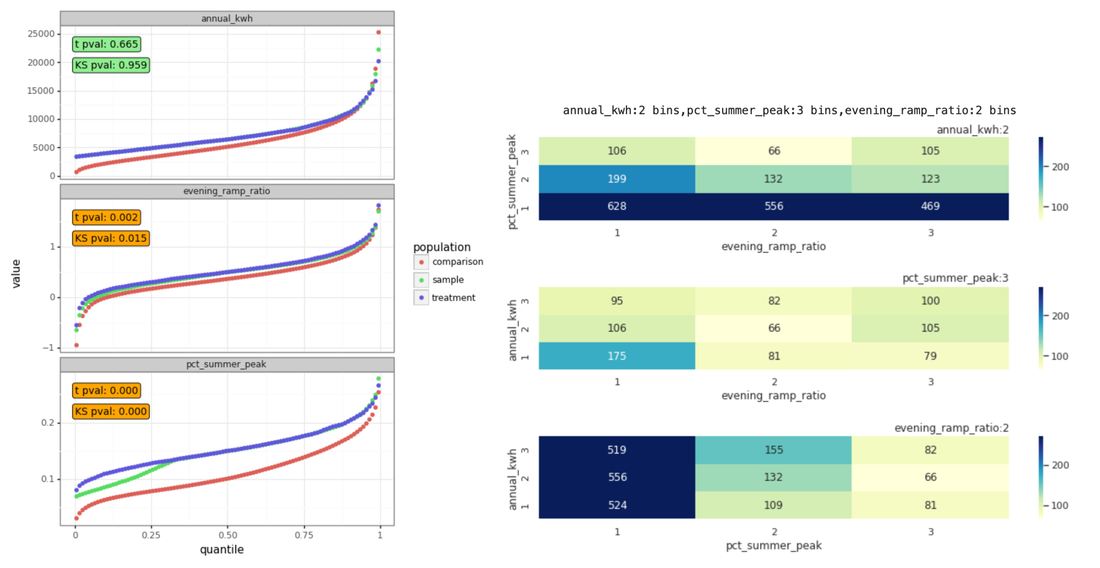
Figure 10: Left: Quantile plots showing the impact of stratification along each parameter that results from the chosen three-dimensional binning scheme Right: Heatmaps that show the sum of squares metric for some of the binning combinations that were searched.
The right-hand plot of Figure 10 are heatmaps that show the sum of squares metric for some of the binning combinations that were searched. Steady improvement can generally be seen from left to right and from bottom to top as the binning is made finer.
Figure 11 shows the full seasonal weekly load shapes for the treatment group, comparison pool, and comparison group. Clear improvement is seen as a result of the stratification and optimization steps.
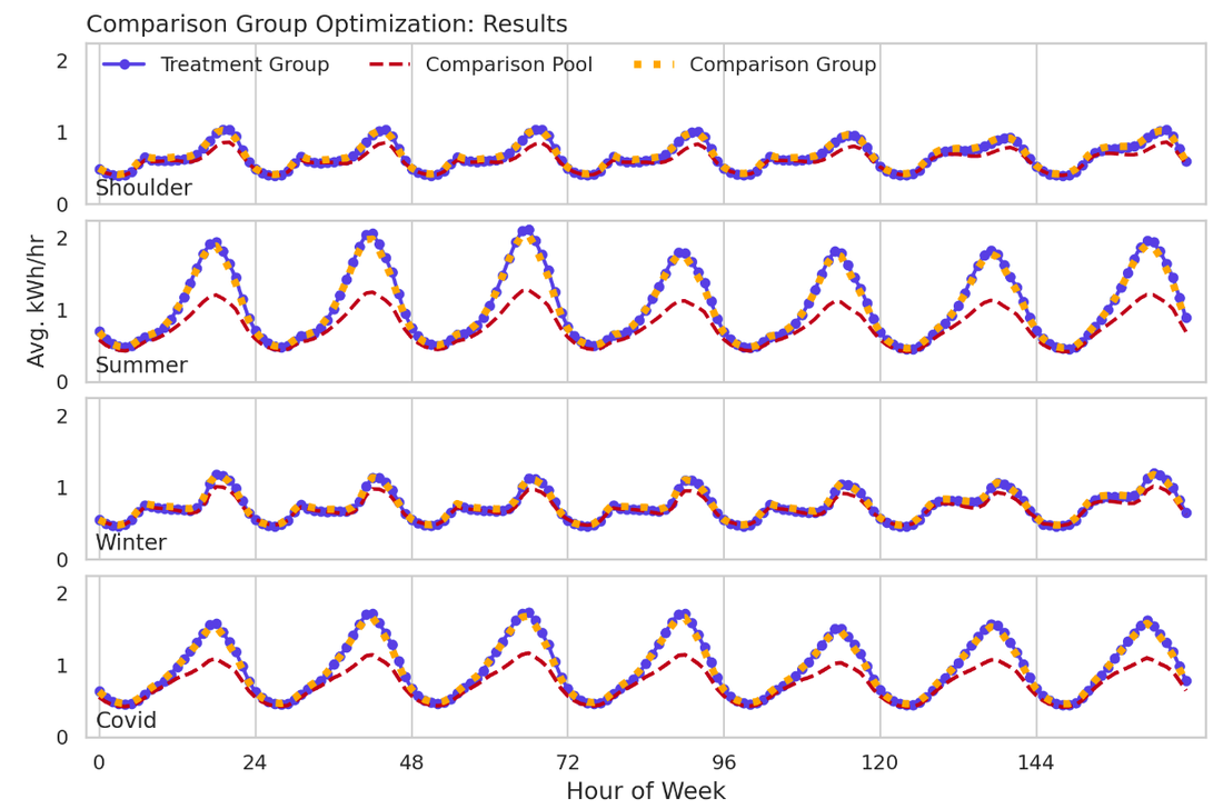
Figure 11: Baseline seasonal weekly load shapes for the treatment group, comparison pool, and comparison group resulting from the advanced stratified sampling scheme described in this chapter.
Just as important a test is how the comparison group behaves during the counterfactual period relative to the treatment group. Figure 12 shows that the good load shape match observed in the baseline period continues into the reporting period (the COVID period).
Just as important a test is how the comparison group behaves during the counterfactual period relative to the treatment group. Figure 12 shows that the good load shape match observed in the baseline period continues into the reporting period (the COVID period).
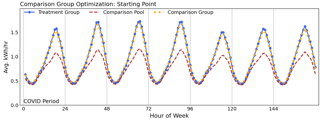
Figure 12: Reporting period (COVID-period) weekly load shapes for the treatment group, comparison pool, and comparison group resulting from the advanced stratified sampling scheme described in this chapter.