Chapter 4:
Difference of Differences Calculations
Introduction
When using a comparison group, the final savings calculation is often referred to as a “difference of differences.” The concept of a difference of differences is relatively straightforward, but if not specified in sufficient detail many different implementations - and answers - are possible. This chapter describes the difference of differences calculation and provides recommendations to specify important implementation details.
The following schematic illustrates the core concept of a difference of differences calculation:
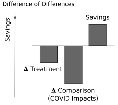
This schematic shows a case in which participant energy usage increased after program intervention. With a comparison group in hand, the difference of differences calculation consists of three basic steps:
1) Measure the change in consumption for program participants. This step is identical to a savings calculation absent a comparison group. In this step a baseline period model is developed for treatment group meters. This model is projected into the reporting period as the counterfactual. The counterfactual is the prediction of energy consumption that would have existed without the program. Subtracting the counterfactual from the actual post-program usage in the treatment group yields a measurement of savings and yields the first “difference” in the difference of differences calculation:
1) Measure the change in consumption for program participants. This step is identical to a savings calculation absent a comparison group. In this step a baseline period model is developed for treatment group meters. This model is projected into the reporting period as the counterfactual. The counterfactual is the prediction of energy consumption that would have existed without the program. Subtracting the counterfactual from the actual post-program usage in the treatment group yields a measurement of savings and yields the first “difference” in the difference of differences calculation:

2) Measure the change in consumption for the comparison group. This step is analogous to step 1 with the measurement conducted on the comparison group. The DifferenceComparison represents the exogenous trends in the broader population and, with a well-designed comparison group, will capture the impacts from COVID and other exogenous factors.2)

3) Compute savings. With the change in consumption figured for both treatment and comparison groups, the program’s impacts are then calculated by adjusting the treatment group savings for the naturally occurring savings observed in the comparison group.
In the schematic above, the treatment group experienced increased usage after program participation. However, the comparison group exhibited an even greater consumption increase, indicating that the program produced positive savings. For residential programs in-field today, this is a very realistic scenario. As described in Chapter 1, Recurve has observed the average residential customer in MCE territory has increased electricity usage by 7.9% on account of COVID. Recurve has observed similar results in the assessment of gas usage for other program administrators. For a program saving 7%, a savings calculation without a comparison group over this same timeframe would yield -1.2% savings.
Figure 13 shows each element of a difference of differences calculation for hypothetical treatment and comparison groups. The curves in the top panel show the observed and counterfactual weekly load shapes of a treatment meter. The difference between the two is calculated and shown as the gray trace. The middle panel gives the same information for the comparison group. Finally, the bottom trace gives the average savings (difference of differences) by hour of the week.
Figure 13 shows each element of a difference of differences calculation for hypothetical treatment and comparison groups. The curves in the top panel show the observed and counterfactual weekly load shapes of a treatment meter. The difference between the two is calculated and shown as the gray trace. The middle panel gives the same information for the comparison group. Finally, the bottom trace gives the average savings (difference of differences) by hour of the week.
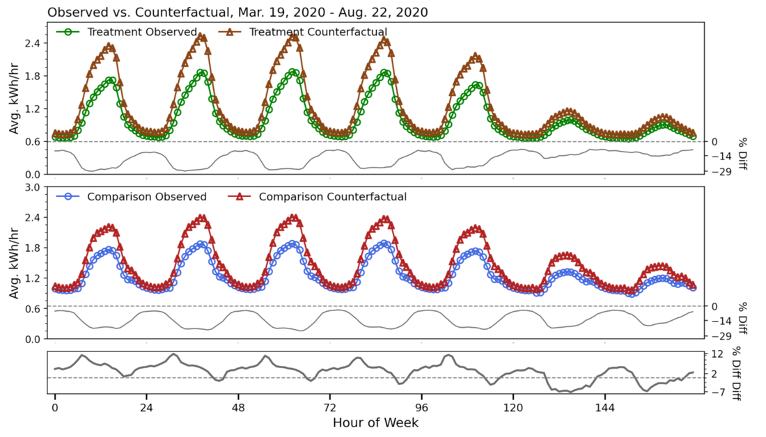
Figure 13: Average weekly load shapes and percent difference traces for each element of a difference of differences calculation for hypothetical treatment and comparison groups
In this example we see that the counterfactual for both the treatment and comparison groups was significantly higher than the observed consumption. This type of scenario is expected to be common for Commercial programs in-field today. Recurve has measured a 15.0% decline in Commercial sector electricity consumption during the COVID period. (See Chapter 1 for more details.)
Program Considerations and Implementation
While the core concepts of a difference of differences calculation are straightforward for those well versed in comparison group theory, in practice several practical questions emerge, including:
Consider the following table, which provides a hypothetical example of a savings calculation for a treatment and comparison group:
In this example we see that the counterfactual for both the treatment and comparison groups was significantly higher than the observed consumption. This type of scenario is expected to be common for Commercial programs in-field today. Recurve has measured a 15.0% decline in Commercial sector electricity consumption during the COVID period. (See Chapter 1 for more details.)
Program Considerations and Implementation
While the core concepts of a difference of differences calculation are straightforward for those well versed in comparison group theory, in practice several practical questions emerge, including:
- Should the difference of differences calculation be conducted on an absolute or percentage basis and why?
- If done on a percentage basis, what value should the resulting percent savings be multiplied by to determine absolute savings?
- How should one account for the staggered project installation dates of a real-world program in determining baseline and “reporting” period dates for the comparison group?
- To mitigate risk and allow for more flexible comparison group selection, the difference of differences calculation should be conducted on a percentage basis.
Consider the following table, which provides a hypothetical example of a savings calculation for a treatment and comparison group:
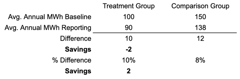
The average treatment group customer used 100 MWh in the baseline period and 90 MWh in the reporting period for a difference of 10 MWh. The average comparison group customer used 150 MWh in the baseline period and 138 MWh in the reporting period for a difference of 12 MWh. If taking the absolute difference of differences we would find that the treatment group customer had negative savings (-2 MWh). However, on a percentage basis, the average treatment group customer used 10% less while the average comparison group customer used 8% less. If savings are calculated via these percentages, we find that a 2% positive savings value should be ascribed to the program.
Importantly, the average comparison group customer was larger than the average treatment group customer. This led to a smaller percentage change in usage producing a larger total change in consumption. While it may be true that the comparison group in this case is clearly not a perfect representation of the treatment group, a program should not be so directly penalized for such a mismatch. With a savings calculation instead conducted on a percentage basis, error from a skewed comparison group is contained to a second-order effect.
While it is important to mitigate risk in the difference of differences calculation by performing the computation on a percentage basis, there is no obvious or perfect answer to the question of what that percentage should ultimately be multiplied by to produce a final savings value. If multiplying by the reporting period observed consumption, the program is penalized for the very savings it produces. If multiplying by the counterfactual, COVID impacts are essentially ignored despite the fact they are obviously real. Multiplying by baseline period usage or the baseline model has the same pitfall. One could envision a hybrid approach in which the percent difference of differences is applied to the combination of treatment group counterfactual adjusted for the COVID impacts observed in the comparison group. However, this level of abstraction introduces unnecessary complexity and does nothing to forward the goal of enabling certainty needed to design and implement meter-based programs.
Here we recommend using the treatment group counterfactual to compute absolute savings from the percent difference of differences calculation. We make this recommendation for two primary reasons:
Energy usage patterns change over time due to economic conditions, changing technologies, population dynamics, and global pandemics, among other factors. The very purpose of a comparison group is to provide a measurement of these exogenous factors that can be immediately applied to best isolate program impacts. For this reason it is important to align the timeline of comparison group calculations to the dates of a program’s participation. As a practical matter this means it is not sufficient to select a comparison group and then simply compute savings for this group for one set of baseline and reporting period dates while the program subject to comparison group adjustment served customers at various points throughout the year. On the other hand, selecting an entirely different comparison group for each week, month, or quarter of a year may be too expensive and impractical. Therefore, as a middle ground, we recommend that at a minimum computing the savings of a single comparison group should be done at multiple points throughout the year to best capture the appropriate timelines for a program. This can be done by producing comparison group savings calculations where the reporting period is set to begin for each month of the year. The savings from these monthly “vintages” of a single comparison group can then be used to adjust treatment group savings via the difference of differences calculation for each monthly cohort of treatment group meters.
The right balance must be struck in the execution of comparison group vintages between temporal granularity and computational cost. Especially when performing hourly calculations on upwards of several thousand comparison group meters, CPU and cloud computing costs as well as the data infrastructure needed to reliably organize and utilize outputs in a transparent manner can become barriers. Along these lines, while the savings calculation is worth the effort to create vintages for the comparison group, for large comparison pools, it is not likely worth the cost to compute all possible stratification parameters, which themselves are derivatives of the baseline period calculation, for every possible baseline across all 12 months of the year. Though some meters may be lost due to data sufficiency requirements from the comparison pool by taking this approach, a reasonably-sized comparison pool should still have a sufficient number of meters available. However, treatment meters should not be discarded for not having a full baseline period available in the year leading up to program launch. For example, a treatment customer who participated in October of 2020 should not be required to have a full 12 months of data from Jan. 1 through Dec. 31 of 2019 to be included in the savings measurement. With these practicalities in mind, we provide the following stepwise approach to implement comparison group vintages for the difference of differences calculation:
Importantly, the average comparison group customer was larger than the average treatment group customer. This led to a smaller percentage change in usage producing a larger total change in consumption. While it may be true that the comparison group in this case is clearly not a perfect representation of the treatment group, a program should not be so directly penalized for such a mismatch. With a savings calculation instead conducted on a percentage basis, error from a skewed comparison group is contained to a second-order effect.
- With a percent difference of differences calculation, final savings should be determined via multiplying by the treatment group counterfactual.
While it is important to mitigate risk in the difference of differences calculation by performing the computation on a percentage basis, there is no obvious or perfect answer to the question of what that percentage should ultimately be multiplied by to produce a final savings value. If multiplying by the reporting period observed consumption, the program is penalized for the very savings it produces. If multiplying by the counterfactual, COVID impacts are essentially ignored despite the fact they are obviously real. Multiplying by baseline period usage or the baseline model has the same pitfall. One could envision a hybrid approach in which the percent difference of differences is applied to the combination of treatment group counterfactual adjusted for the COVID impacts observed in the comparison group. However, this level of abstraction introduces unnecessary complexity and does nothing to forward the goal of enabling certainty needed to design and implement meter-based programs.
Here we recommend using the treatment group counterfactual to compute absolute savings from the percent difference of differences calculation. We make this recommendation for two primary reasons:
- This would be the most sensible and justifiable approach in the absence of a large exogenous event like COVID. As time goes on, COVID impacts should diminish (we already see evidence that COVID impacts have abated over the last several months in MCE data and elsewhere) and this choice is therefore most appropriate for the long term.
- Most program interventions produce savings with expected persistence of several years or more. The “lifecycle” savings that result from a meter-based measurement are often determined by applying the first-year savings calculation across the expected lifetime of the measure. For longer-lived program impacts using the treatment group counterfactual can help ensure the first-year savings measurement is most appropriate for application to a lifecycle savings calculation, despite COVID.
- Baseline and reporting period comparison group calculations should closely mirror the range of treatment group intervention dates.
Energy usage patterns change over time due to economic conditions, changing technologies, population dynamics, and global pandemics, among other factors. The very purpose of a comparison group is to provide a measurement of these exogenous factors that can be immediately applied to best isolate program impacts. For this reason it is important to align the timeline of comparison group calculations to the dates of a program’s participation. As a practical matter this means it is not sufficient to select a comparison group and then simply compute savings for this group for one set of baseline and reporting period dates while the program subject to comparison group adjustment served customers at various points throughout the year. On the other hand, selecting an entirely different comparison group for each week, month, or quarter of a year may be too expensive and impractical. Therefore, as a middle ground, we recommend that at a minimum computing the savings of a single comparison group should be done at multiple points throughout the year to best capture the appropriate timelines for a program. This can be done by producing comparison group savings calculations where the reporting period is set to begin for each month of the year. The savings from these monthly “vintages” of a single comparison group can then be used to adjust treatment group savings via the difference of differences calculation for each monthly cohort of treatment group meters.
The right balance must be struck in the execution of comparison group vintages between temporal granularity and computational cost. Especially when performing hourly calculations on upwards of several thousand comparison group meters, CPU and cloud computing costs as well as the data infrastructure needed to reliably organize and utilize outputs in a transparent manner can become barriers. Along these lines, while the savings calculation is worth the effort to create vintages for the comparison group, for large comparison pools, it is not likely worth the cost to compute all possible stratification parameters, which themselves are derivatives of the baseline period calculation, for every possible baseline across all 12 months of the year. Though some meters may be lost due to data sufficiency requirements from the comparison pool by taking this approach, a reasonably-sized comparison pool should still have a sufficient number of meters available. However, treatment meters should not be discarded for not having a full baseline period available in the year leading up to program launch. For example, a treatment customer who participated in October of 2020 should not be required to have a full 12 months of data from Jan. 1 through Dec. 31 of 2019 to be included in the savings measurement. With these practicalities in mind, we provide the following stepwise approach to implement comparison group vintages for the difference of differences calculation:
- If using stratified sampling or proportional sampling based on usage characteristics as described in Chapter 3, complete steps i and v. If using random sampling or proportional sampling based on geography alone, steps i and v can be skipped.
- Using the 12 months preceding the program year as a baseline period, compute stratification parameters for the entire comparison pool.
- Compute monthly, daily or hourly savings depending on the granularity of consumption data for all meters in the treatment group per CalTRACK 2.0 methods.
- Assign each treatment meter to a monthly cohort according to its program participation end date.
- Compute percent savings for each treatment group monthly cohort:

where the summations are computed over all treatment group meters. This is done on an hourly, daily, or monthly basis depending on the granularity of the consumption data. The monthly cohort is determined by the program intervention end date.
- With the same baseline periods utilized for step ii, compute stratification parameters for each member of the treatment group. (Note that several important stratification parameters, including heating and cooling loads are derived from outputs of CalTRACK calculations.)
- Complete comparison group sampling as detailed in Chapter 3.
- Compute savings using CalTRACK 2.0 methods for the comparison group for each monthly vintage. The baseline period for the first vintage will consist of the 365 days leading up to the first month of the program year. The reporting period for the first vintage will begin on the first day of the month beginning the program year and run for the subsequent 365 days. For instance, for a program year beginning in Jan. 2021, compute comparison group savings using CalTRACK 2.0 methods with a baseline period of Jan. 1, 2019 - Dec. 31, 2019 and a reporting period of Jan. 1, 2020 - Dec. 31, 2020. The second vintage will be shifted exactly 1 month forward for both baseline and reporting periods. This step is complete when comparison group savings are computed for all 12 monthly vintages.
- Compute savings for all comparison group monthly vintages:

where i indicates the monthly vintage and the summations are computed over all comparison group meters. This is done on an hourly, daily, or monthly basis depending on the granularity of the consumption data.
- For each monthly cohort compute the percent difference of differences:

This is done on an hourly, daily, or monthly basis depending on the granularity of the consumption data.
- Compute monthly cohort savings by multiplying the percent difference of differences by the treatment group counterfactual:

This is done on an hourly, daily, or monthly basis depending on the granularity of the consumption data.
- Compute total hourly, daily, monthly, or annual savings by summing results from all monthly cohorts as needed.